Apply a window

In signal processing and statistics, a window function (also known as an apodization function or tapering function) is a mathematical function that is zero-valued outside of some chosen interval, normally symmetric around the middle of the interval, usually near a maximum in the middle, and usually tapering away from the middle. Mathematically, when another function or waveform/data-sequence is “multiplied” by a window function, the product is also zero-valued outside the interval: all that is left is the part where they overlap, the “view through the window”.

Source: Wikipedia

A sound waveform might have an abrupt onset or offset. It is often preferred to apply a window to ramp up and ramp down the volume.

import numpy as np
from matplotlib import pyplot as plt
from scipy.signal.windows import tukey

from stimuli.audio import Tone

In this tutorial, we will create a pure tone auditory stimuli and apply a window with a linear ramp-up and a linear ramp-down to smooth the onset and offset.

Create a pure tone

To create the stimuli, we create a Tone object with a given volume and frequency.

sound = Tone(volume=10, frequency=200, duration=0.1)

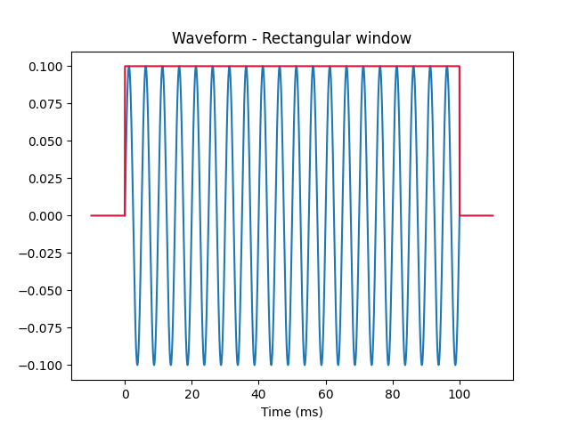
By default, a generated signal will have a rectangular window applied. A recctangular window is equal to 0 outside of the signal definition range, and to 1 inside. We can plot the waveform of one of the channels:

# draw the waveform
plt.figure()
plt.plot(sound.times * 1000, sound.signal[:, 0])
plt.xlabel("Time (ms)")
plt.title("Waveform - Rectangular window")

# overlay a rectangular window
# note: for demonstration purposes, we make the window 20% longer than the
# signal by extending it by 10% before and after the signal.
extension = int(0.1 * sound.n_samples)
window = np.zeros(extension + sound.n_samples + extension)
window[extension + 1 : extension + sound.n_samples] = 1 / sound.volume
# determine the timestamps associated to each sample in the window (ms)
window_times = np.arange(
    0, 1 / sound.sample_rate * window.size, 1 / sound.sample_rate
)
window_times -= extension / sound.sample_rate
window_times *= 1000
# draw the window
plt.plot(window_times, window, color="crimson")
plt.show()

Create a different window

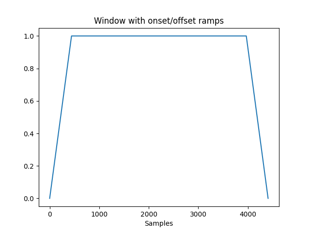
For this tutorial, we will define a window with a ramp from 0 to 1 during the first 10% of the total duration, and a ramp from 1 to 0 during the last 10% of the total duration. A correctly defined window is a 1D array with the same number of samples as the sound.

window = np.ones(sound.n_samples)
n_samples_ramp = int(0.1 * sound.n_samples)
ramp = np.linspace(start=0, stop=1, num=n_samples_ramp)
window[:n_samples_ramp] = ramp
window[-n_samples_ramp:] = ramp[::-1]

# draw the window
plt.figure()
plt.plot(window)
plt.title("Window with onset/offset ramps")
plt.xlabel("Samples")
plt.show()

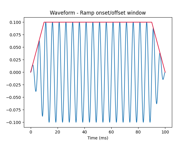
Change the window

We can change the applied window by setting the attribute window.

sound.window = window

# draw the modified sound and the window
plt.figure()
plt.plot(sound.times * 1000, sound.signal[:, 0])
plt.xlabel("Time (ms)")
plt.title("Waveform - Ramp onset/offset window")

# overlay the window
plt.plot(sound.times * 1000, window / sound.volume, color="crimson")
plt.show()

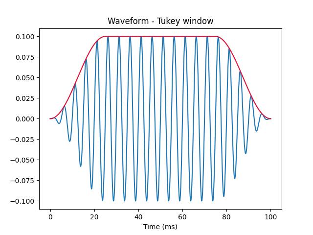
Scipy windows

scipy has many windows implemented in scipy.signal.windows. For instance we can use a Tukey window with the function tukey.

window = tukey(sound.n_samples)
sound.window = window

# draw the modified sound and the window
plt.figure()
plt.plot(sound.times * 1000, sound.signal[:, 0])
plt.xlabel("Time (ms)")
plt.title("Waveform - Tukey window")

# overlay the window
plt.plot(sound.times * 1000, window / sound.volume, color="crimson")
plt.show()

Estimated memory usage: 36 MB