Base sounds

stimuli provides a common API for audio stimuli. The audio stimuli can be either generated or loaded. A generated stimuli can be exported. The volume, duration and other properties can be set when creating the stimuli or updated between plays.

from pathlib import Path
from tempfile import TemporaryDirectory

from matplotlib import pyplot as plt

from stimuli.audio import Sound, Tone

In this tutorial, we will create, edit, save and load a pure tone auditory stimuli. A pure tone is a signal with a sinusoidal waveform, that is a sine wave of any frequency, phase-shift and amplitude.

Source: Wikipedia

Create and edit a pure tone

To create the stimuli, we create a Tone object with a given volume and frequency.

sound = Tone(frequency=440, volume=10, duration=0.1)  # La - A440

We can listen to the sound we created with play().

sound.play(blocking=True)

We can edit the sound properties by replacing the value in the properties. For instance, let’s increase the volume and change the frequency.

sound.volume = 50  # percentage between 0 and 100
sound.frequency = 1000  # Hz

The sound is updated each time an attribute is changed.

sound.play(blocking=True)

Export/Load a sound

We can export a sound with save() and load a sound with Sound.

with TemporaryDirectory() as directory:
    fname = Path(directory) / "my_pure_tone.wav"
    sound.save(fname, overwrite=True)
    sound_loaded = Sound(fname)
sound_loaded.play(blocking=True)

However, a loaded sound can be any type of sound. stimuli does not know that the sound was exported with the save() method of one of its class. As such, the attributes that were specific to the original sound are not present anymore and can not be updated anymore.

print(hasattr(sound_loaded, "frequency"))

False

Only the basic attributes are preserved: duration, sample_rate.

print(f"Duration of the original sound: {sound.duration} second.")
print(f"Duration of the loaded sound: {sound_loaded.duration} second.")
print(f"Sample rate of the original sound: {sound.sample_rate} Hz.")
print(f"Sample rate of the loaded sound: {sound_loaded.sample_rate} Hz.")

Duration of the original sound: 0.1 second.
Duration of the loaded sound: 0.1 second.
Sample rate of the original sound: 44100 Hz.
Sample rate of the loaded sound: 44100 Hz.

The volume is normalized, with the loudest channel set to 100. The ratio between channels is preserved.

print(f"Volume of the original sound: {sound.volume}.")
print(f"Volume of the loaded sound: {sound_loaded.volume}.")

Volume of the original sound: [50.].
Volume of the loaded sound: [100.].

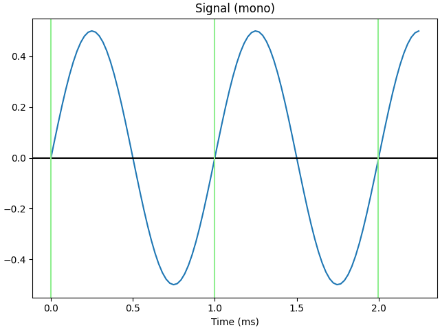
Visualize a sound

Finally, the underlying signal is stored in the signal property, a numpy array of shape (n_samples, n_channels). We can plot the signal of each channel.

samples_to_plot = 100  # number of samples to plot
times = sound.times[:samples_to_plot] * 1000  # ms

f, ax = plt.subplots(1, 1, layout="constrained")
ax.plot(times, sound.signal.squeeze()[:samples_to_plot])  # draw data
ax.axhline(0, color="black")  # draw horizontal line through y=0

# labels
ax.set_title("Signal (mono)")
ax.set_xlabel("Time (ms)")

# draw vertical line after each period
period = int(sound.sample_rate / sound.frequency)
for k in range(0, samples_to_plot, period):
    ax.axvline(times[k], color="lightgreen")

plt.show()

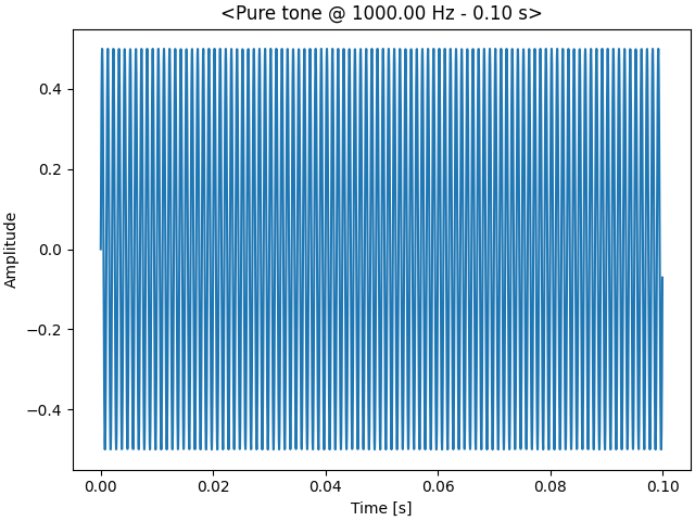
Or with the convenient plot() method.

sound.plot()
plt.show()

Estimated memory usage: 158 MB